

Statistical Analysis:
Understanding Statistical Distributions
See also: Significance and Confidence Intervals
Over many years, eminent statisticians noticed that data from samples and populations often formed very similar patterns. For example, a lot of data were grouped around the ‘middle’ values, with fewer observations at the outside edges of the distribution (very high or very low values). These patterns are known as ‘distributions’, because they describe how the data are ‘distributed’ across the range of possible values.
Mathematicians have developed standard statistical distributions that describe these patterns. These standard statistical distributions are often used in statistical analysis as reference distributions. This means that they allow researchers to compare data and groups of samples more easily.
This page describes some of the standard distributions, and explains their importance in statistical testing.
The Normal Distribution
The normal distribution is perhaps the best-known statistical distribution, and it looks like this:
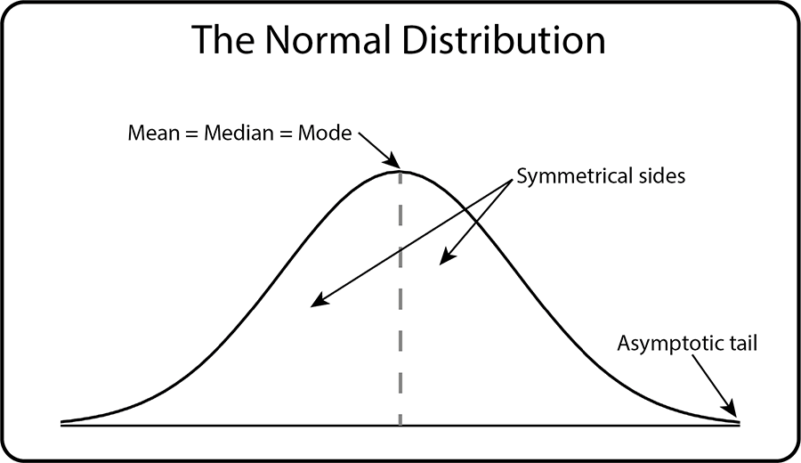
It is also known as the bell curve, because of its shape, and the Gaussian distribution after the mathematician Carl F Gauss, who first described it.
It is a distribution of continuous variables, where data can take an infinite number of values between any two values (for more about this, see our page on Types of Data).
Close approximations to the normal distribution are widely found in nature, especially biology. For example, heights, weights and blood pressure tend to follow this shape of distribution in the population, with a cluster around the middle, tailing off towards either side (very high and very low values). The tails are asymptotic, or infinite, tending towards, but never reaching, zero probability.
It is also important because many of the most powerful statistical tests require the data to be normal. These include the Pearson product-moment correlation test (for more about this, see our page on Statistical Analysis: Understanding Correlations).
The normal curve also has some useful characteristics related to probability and standard deviation (a measure of how widely the data are spread around the mean). For more about standard deviation, see our page on Simple Statistical Analysis.
For example:
68% of values are within one standard deviation (SD) either side of the mean (sometimes written as ±1 SD):

You therefore have a 68% chance of randomly selecting a data point that is within one standard deviation of the mean.
95% of values are within two standard deviations either side of the mean (±2 SD):
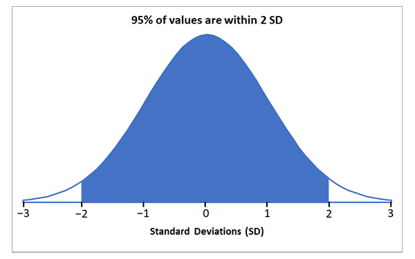
This means that you have a 95% chance of randomly selecting a data point that is within two standard deviations of the mean.
99.7% of values are within three standard deviations of the mean (±3 SD):
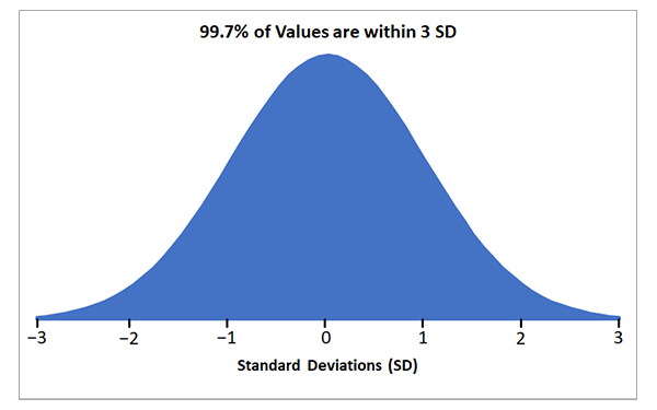
If you select a data point at random, there is a 99.7% chance that it will be within three standard deviations of the mean.
You can test whether your data follow a normal distribution using statistical tests such as the Kolmogorov–Smirnov test or the Shapiro–Wilk test (statistical software packages will calculate these automatically for you). An insignificant result tells you that your data are normally distributed.
You can find out more about significance tests in our page on Significance Testing and Confidence Intervals.
A Special Case: the t-Distribution
The t-distribution is the same as the normal distribution. However, when it is used as a reference distribution in statistical testing, the standard deviation of the reference data is estimated from the sample data, rather than given as standard.
Binomial and Poisson Distributions
The binomial and Poisson distributions are both discrete probability distributions. In other words, they describe the distribution of the probability of particular events happening.
The binomial distribution is the discrete probability distribution of the number of successes in a sequence of independent experiments, each with a yes/no (or true/false) outcome. It can therefore be used, for example, for the probability of drawing an ace from a pack of cards, if the card is replaced after each draw, or for throwing a particular value on a dice.
Unlike the normal distribution, the binomial distribution can be shown as a histogram:

The graph above shows the distribution of the chances of a coin toss giving a tail (a probability of 50% or p = 0.5) in ten tests (n = 10). In other words, if you carried out 10 coin tosses about 100 times, you would get a distribution something like this: you would get five tails most often, around 24% of the time, followed by four and six around 20% of the time, and so on.
The Poisson distribution shows the probability of a given number of events occurring in a given time period. It is therefore a particular case of the binomial distribution, and is widely used for stock trading (where there is no trading below a certain level, but the maximum value is technically infinite). It is also suitable for looking at radioactive decay. It is less symmetrical than the standard binomial distribution, with a longer tail at the upper end of values:

Other Statistical Distributions
There are several other statistical distributions that are used in statistical testing, all with slightly different parameters. They include:
- The chi-square (χ2) distribution, which is the distribution of variances, rather than variable values or means (like the distributions previously described);
- The F-distribution, which is the distribution of ratios of variances.
Characteristics of Standard Distributions
Standard distributions share a number of characteristics. These characteristics include:
A clear mathematical definition. Their shape reflects just a few parameters, such as mean and standard deviation (for the normal distribution) or variance (for the chi-squared distribution).
Established theoretical properties. We know a lot about these distributions (for example, the normal curve is symmetrical).
They are good estimations for real data. In a sample of real-world data, it is impossible to get an exact normal distribution. However, these distributions are very good approximations of real data.
Using Standard Distributions as Reference Distributions
Standard distributions are often used as reference distributions in statistical testing.
This means that sample data are compared with them to see how likely it is that the data have occurred at random.
The characteristics of standard distributions make them very suitable to be reference distributions, especially the well-known characteristics, and the fact that they are good approximations of real-world data.
However, there are other sources of reference distributions.
Bootstrap distributions are created by assuming that the sample data are the only data available, and drawing repeated (smaller) samples from those data. These can only really be used when you have access to a computer, and are not ideal. They should therefore only be used when there is no alternative.
Permutational distributions are created by finding all the possible permutations of ranked data. They therefore take all the possible outcomes and see how likely they are. They do not assume any underlying theoretical distribution. Tests using these distributions are known as ‘non-parametric’ tests, to distinguish them from the ‘parametric’ tests that use standard distributions with known parameters.
Archive data can also be used to create a reference distribution. This may be appropriate where there are a lot of past data that can be used.
Why Statistical Distributions Matter
The main reason why you need to understand about statistical distributions is their use in statistical testing.
You can use them to compare your data, to help you understand how likely it is that you have identified a real relationship or feature from your data.